Introduction to Machine Learning

Introduction

• ML is an intersection of data science and software engineering.
• The goal of ML is to use data to create a predictive model that can be incorporated into a software application or service.
• This goal requires the collaboration of Data Scientists and Software Developer.
• Data Scientists explores and prepares the data before using it to train a machine learning model.
• Software Developers integrated the models into applications where they are used to predict new data values. This process is known as inferencing.

What is Machine Learning?

• ML has its origins in statistics and mathematical modeling of data.
• The idea of ML is to use the data from past observations to predict unknown outcomes or values.

For Example:

• The proprietor of an ice cream store might use an app that combines historical sales and weather records to predict how many ice creams they are likely to sell on a given day, based on the weather forecast.

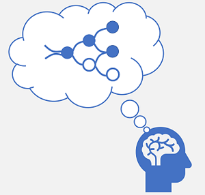
Machine Learning as a function

• Since ML originates from mathematics and statistics, its a common way to think about ML models in mathematical terms.
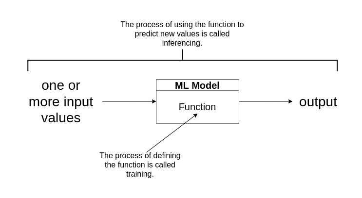
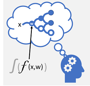
• A ML model is a software application that encapsulates a function to calculate an output value based on one of more input values.
• The process of defining this function is known as training.
• After the function has been defined, the process of using it to predict new values is called inferencing.

Steps involved in training and inferencing

1. The training data consists of past observations. In most cases the observations include:

   1. Attributes/Features of the thing being observed.

   2. Known value of the thing, a.k.a. Label.

      For example

      The observed data in the dataset used to predict house prices includes attributes/features such as size, number of bedrooms, location and age of the house; while the known value/label in this case will be the selling price of the house. Once the model is trained, it can analyze new houses with similar features to predict their prices.

      In mathematical terms, the features are often referred to using the shorthand variable name $x$, and the label referred to as $y$. Usually, an observation consists of multiple features values; hence, x is actually a vector (an array with multiple values) like $[x1, x2, x3]$.

      For example

      In the ice cream sales scenario, our goal is to train a model that can predict the number of ice cream sales based on the weather. The weather measurements for the day (temperature, rainfall, windspeed, and so on) would be the features (x), and the number of ice creams sold on each day would be the label (y).

2. An algorithm is applied to the data to try to determine a relationship between the features and label and generalize that relationship as a calculation that can be performed on $x$ to calculate $y$. The basic principle is to try to fit the data to a function in which the values of the features can be used to calculate the label.

3. The result of the algorithm is a model that encapsulates the calculation derived by the algorithm as a function. Lets call it f. In mathematical notation:

   $y = f(x)$

4. After this training phase, the trained model can be used for inferencing. You can input a set of feature values, and receive as an output a prediction of the corresponding label. Because the output from the model is a prediction that was calculated by the function, and not an observed value, you will often see the output from the function shown as $\hat{y}$.

Types of Machine Learning

There are multiple types of machine learning, and you must apply the appropriate type depending on what you are trying to predict. A breakdown of common types of machine learning is shown in the following diagram.

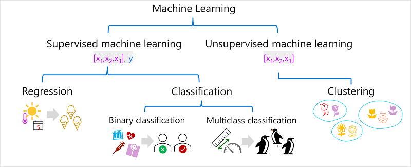
Supervised Machine Learning

• Supervised ML is a term for ML algorithm in which the training data includes both, the feature values and known label values.
• It is used to train models by determining a relationship between the features and labels in past observations.
• This helps the model to predict the unknown labels for the known features.

Regression

• Regression is a form of supervised ML in which the label predicted by the model is a numeric value.

For Example

• The number of ice creams sold on a given day, based on the temperature, rainfall, and windspeed.

Classification

• Classification is a form of supervised ML in which the label represents a categorization or class.

Binary Classification

• Binary classification predicts the outcome in boolean. The predicted label can be either true/false or positive/negative.

For Example

• Whether a patient is at risk for diabetes based on clinical metrics like weight, age, blood glucose level, and so on.

Multiclass Classification

• Multiclass Classification extends binary classification to predict a label that represents one of multiple possible classes.

For Example

• The genre of a movie (comedy, horror, romance, adventure, or science fiction) based on its cast, director, and budget.

• In most scenarios that involve a known set of multiple classes, multiclass classification is used to predict mutually exclusive labels.

• For example, a penguin can't be both a Gentoo and an Adelie.

• However, there are also some algorithms that you can use to train multilabel classification models, in which there may be more than one valid label for a single observation.

• For example, a movie could potentially be categorized as both science fiction and comedy.

Unsupervised Machine Learning

• Unsupervised ML is an algorithm in which the training data only includes the feature values but no known labels.
• It determines the relationships between the features of the observations in the training data.

Clustering

• Clustering is an algorithm that identifies the similarities between observations based on the features and groups them into discrete clusters.
• The most common form of unsupervised ML is clustering.

For example

• Group similar flowers based on their size, number of leaves, and number of petals.

• In some cases, clustering is used to determine the set of classes that exists.

• Then these classes can act as label of the observations which can be used to train classification model.

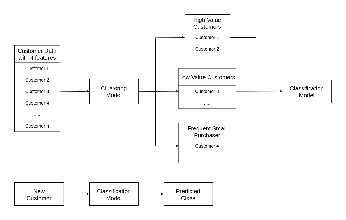
For example

• You have observation of all the customers without any labels.
• You can first use clustering to segment the customers into groups, analyze the groups to identify and categorize different classes of customers.
• Now you have the observation along with the label (that is the class in which each observation belongs).
• You can use this labeled observations to train a classification model.
• This model can be further used to predict the class in which the new customer belongs.

Regression

• Regression models are trained to predict the label values based on the training data.
• The training data includes both features and known labels.
• The process for training any supervised ML model involves multiple iterations in which you use an appropriate algorithm to train a model usually with some parameterized settings, evaluate the predictive performance and refine the model by repeating the training process with different algorithms and parameters, until you achieve an acceptable level of predictive accuracy.

Understanding algorithm and its elements

• Consider the first algorithm to be $\mathcal{Y} = \beta_0 + \beta_1\mathcal{X} + \varepsilon$. In this algorithm, y is the predictive label and $\beta_0 + \beta_1\mathcal{X} + \varepsilon$ is the algorithm including $\beta_0$ and $\beta_1$ as parameters.

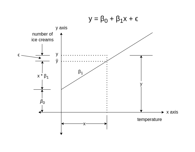
• The value of $\mathcal{Y}$ (prediction) will increase/decrease as the value of $x$ (features) increases.
• Hence, $\mathcal{Y}$ is either directly or inversely proportional to $x$.
• In our case, the value of number of ice creams will increase with the increase in temperature.
• Therefore, $\mathcal{Y}\propto\mathcal{X}$.
• Therefore, $\mathcal{Y} = \beta_1 \times \mathcal{X}$; where
  • $\beta_1$ = constant of proportionality. Also called the slope of the line describing the relationship between $\mathcal{Y}$ and $\mathcal{X}$.
• Further, there might a starting point at which the value of $\mathcal{Y}$ starts.
• In our case, we can call it the base value or the number of ice creams that are sold regardless of the temperature. This value can also be 0.
• Lets represent this value by $\beta_0$.
• It is the y-intercept of the line.
• Now the equation becomes $\mathcal{Y} = \beta_0 + \beta_1\mathcal{X} + \varepsilon$; where
  • $\varepsilon$ = The difference between the predicted label and the actual label of the feature.

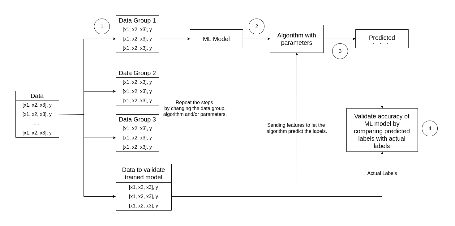
Four key elements of training process for supervised ML model

Step 1

1. Randomly split the training data into multiple groups.
2. This creates various groups of data which can be used to train the model.
3. Hold back a group of data that can be further used to validate the trained model.

Step 2

1. Use an algorithm to fit the training data into a model.
2. In case of a regression model, use a regression algorithm such as linear regression. In the above example, linear regression is used to explain all the element of the algorithm.

Step 3

1. Use the group of data that we held, to validate the model by letting it predict the labels for the features.

Step 4

1. Compare the known actual labels in the group of data, with the labels that model predicted.
2. Then aggregate the differences between the predicted and actual label, to calculate a metric that indicates how accurately the model predicted for the validation data.

• After each train, validate and evaluate iteration.
• You can repeat the process with different algorithms and parameters, until an acceptable evaluation metric is achieved.

To understand all the steps and actions with a practical example, please check this page on Microsoft Learn. It walks through each step along with a sample data to demonstrate the concept.

Regression evaluation metrics

• Based on the predicted and actual values, you can calculate some common metrics that are used to evaluate a regression model.
• For understanding each metrics, consider the following observations for the ice cream sales.

Temperature ($\mathcal{X}$)	Actual sales ($\mathcal{Y}$)	Predicted sales ($\hat{\mathcal{Y}}$)	Difference ($\lvert\hat{\mathcal{Y}} - \mathcal{Y}\lvert$)
52	0	2	2
67	14	17	3
70	23	20	3
73	22	23	1
78	26	28	2
83	36	33	3

Mean Absolute Error (MAE)

• To calculate MAE, we need to get the unit different between the actual label and predicted label for each observation.
• This difference is absolute. Hence, it doesnt matter if the actual label is above the predicted label or below.
• For example, both the differences, that is, -3 and +3, will be considered 3.
• The value of MAE is the average of all the absolute differences.
• Hence, the name Mean Absolute Error.
• In the ice cream example, the mean (average) of the absolute errors (2, 3, 3, 1, 2, and 3) is 2.33.

Mean Squared Error (MSE)

• The Mean Absolute Error takes into account, all the discrepancies between the predicted and actual labels equally.
• However, it is more desirable to have a model that consistently makes small errors vs a model that makes fewer but large errors.
• One way of getting that metrics that amplifies the large errors is by squaring the individual errors and calculating the mean of the squared values.
• This metric is known as Mean Squared Error.
• In our ice cream example, the mean of the squared absolute values (which are 4, 9, 9, 1, 4, and 9) is 6.

Root Mean Squared Error (RMSE)

• The Mean Squared Error helps take the magnitude of errors into account, but because it squares the error values, the resulting metric no longer represents the quantity measured by the label.
• To get the error in terms of the unit of label, we need to calculate the square root of MSE.
• It produces a metric called Root Mean Squared Error.
• In this case √6, which is 2.45 (ice creams).

Coefficient of determination ($R^2$)

• All the metrics so far, compare the discrepancy between the predicted and the actual value in order to evaluate the model. However, in reality, there is some natural random variance in the daily data that model takes into account.
• To find the natural variation existing in each data, we need to have a reference point.
• This reference point can be the average of all the data.
• Using this reference point, we can calculate the variation that exist in the data.
• In this case, the average of the actual sales is $\approx20.167$.
• Now the absolute variation in each data can be calculated as 20.167, 6.167, 3.167, 2.167, 6.167 and 16.167.
• Now we will find the RMS value of these data due to the same reasons as mentioned in Mean Square Error description.
• The RMS value of the data is $\approx11.25$.
• This is the variation that already exists in the data.
• Now, we need to find the variation in the predicted data and the actual data.
• For this one we do not need a reference value because we already have 2 entities.
• The absolute variation in the data predicted by the model is 2, 3, 3, 1, 2, 3.
• This was a simple calculation.
• The RMS value of this variation is 2.45.
• Now, the actual (or ideal) variation in the data is 11.25 and the total variation by the model is 2.45.
• If we remove the total variation by the model from the actual variation in the data, we get 11.25 - 2.45 = 8.8.
• This is the proportion of the variation from the actual variation that we can get from the model.
• Hence, to calculate how well the model explains the data, we divide the variation the model is able to capture (which is 11.25−2.45=8.8) by the total variation in the data (which is 11.25).
• The value that we get, indicates how accurate the model is.
• This value is call the coefficient of determination, which ranges between 0 to 1.
• 1 indicates that the model is efficiently able to get the variation that already exists in the data; while 0 indicates that the model is inefficient and it is only able to guess the mean.

Iterative Training

• All the metrics explained above are used to evaluate a regression model.
• A data scientist uses an iterative approach to repeatedly train and evaluate a model, varying:
  • Feature Selection and Preparation: Choosing which features to include in the model, and calculations applied to them to help ensure a better fit.
  • Algorithm selection: There are many regression algorithms
  • Algorithm parameters: In case of linear regression algorithm, the parameters were $\beta_0, \beta_1$ etc. However, in general parameters means the coefficients that represents the relationship between the features and the predicted value of labels.

Binary Classification

• Since classification is also a supervised ML technique, it follows the same iterative process of training, validating and evaluating models.
• Instead of calculating the numeric values using the features like regression model, the algorithms used to train classification models calculate probability values that decides the class to which the features belong.
• The evaluation metrics used to access the model performance, compare the predicted classes to the actual classes.
• Binary classification algorithms are used to train a model that predicts one of the two possible tables for a single class, as the name suggests.
• In most real world scenarios, the data observations used to train and validate the model consists of multiple feature ($\mathcal{X}$) values and a $\mathcal{Y}$ value that is either 1 or 0.

Sample Data

• Consider the following sample data having a single feature $\mathcal{X}$ to predict whether the label $\mathcal{Y}$ is 1 or 0.
• In the example, we use the blood glucose level of patients to predict if the patient has diabetes.

Blood glucose (x)	Diabetic? (y)
67	0
103	1
114	1
72	0
116	1
65	0

Training a binary classification model

• To train the model, we will use an algorithm to fit the training data to a function that calculates the probability of the class label being true. That is if the patient has diabetes.
• Probability is measured as a value between 0 and 1, such that the total probability for all the possible classes is 1.
• For example, if the probability of a patient having diabetes is 0.7, then there is a corresponding probability of 0.3 that the patient is not diabetic.
• There are many algorithm that can be used for binary classification, such as logistic regression, which derives a sigmoid (S-shaped) function with values between 0 and 1, like this:

note

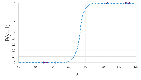
Despite its name, in machine learning logistic regression is used for classification, not regression. The important point is the logistic nature of the function it produces, which describes an S-shaped curve between a lower and upper value (0.0 and 1.0 when used for binary classification).

• The function produced by the algorithm describes the probability of $\mathcal{Y}$ being true ($\mathcal{Y}$ = 1) for a given value of $\mathcal{X}$.
• Mathematically, you can express the function like this: $$f(\mathcal{X}) = P(\mathcal{Y}=1 | \mathcal{X})$$
• For the three of the six observations in the training data, we know that $\mathcal{Y}$ is definitely true, so the probability for those observations that $\mathcal{Y} = 1$ is 1 and for the other three, we know that $\mathcal{Y}$ is definitely false, so the probability that $\mathcal{Y} = 1$ is 0.
• The S-shaped curve describes the probability distribution, so that plotting a value of $\mathcal{X}$ on the line identifies the corresponding probability of $\mathcal{Y} = 1$.
• The diagram includes a horizontal line to indicate the threshold at which a model based on this function will predict true or false.
• The threshold lies at the mid-point for $\mathcal{Y}$ $(P(\mathcal{Y}) = 0.5)$ .
• For any values at this point or above, the model will predict true; while for any values below this point it will predict false.
• For example for a patient with blood glucose level 90, the function would result in a probability value of 0.9.
• Since 0.9 is higher than the threshold of 0.5, the model would predict true.
• In other words, the patient is predicted to have diabetes.

Evaluating a binary classification model

• Assuming the following data were held to validate the trained model.

Blood glucose (x)	Diabetic? (y)
66	0
107	1
112	1
71	0
87	1
89	1

• Applying the logistic function we derived previously to the $\mathcal{X}$ values results in the following plot.

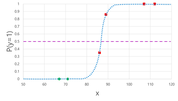
• Based on whether the probability calculated by the function is above or below the threshold, the model generates a predicted label of 1 or 0 for each observation.
• Following is the comparison of predicted class labels ($\hat{\mathcal{Y}}$) to the actual class labels ($\mathcal{Y}$).

Blood glucose (x)	Actual diabetes diagnosis (y)	Predicted diabetes diagnosis (ŷ)
66	0	0
107	1	1
112	1	1
71	0	0
87	1	0
89	1	1

Binary classification evaluation metrics

• The first step in evaluation metrics for a binary classification models is usually to create a matrix of the number of correct and incorrect predictions for each possible class label.

• This visualization is known as confusion matrix and it shows prediction totals where:
  • ŷ=0 and y=0: True negatives (TN)
  • ŷ=1 and y=0: False positives (FP)
  • ŷ=0 and y=1: False negatives (FN)
  • ŷ=1 and y=1: True positives (TP)
• The arrangement of the confusion matrix is such that correct (true) predictions are shown in a diagonal line from top-left to bottom-right.
• Often, color-intensity is used to indicate the number of predictions in each cell, so a quick glance at a model that predicts well should reveal a deeply shaded diagonal trend.

Accuracy

• This is the simplest metric that you can calculate from the confusion matrix is accuracy.
• It can be calculated by dividing total right predictions from total predictions.
• More formally formulated (TN + TP) / (TN + FN + TP + FP)
• In our case, the calculation is 5 / 6 = 0.83.
• Hence, for our validation data, the classification model produced correct predictions 83% of the time.
• Accuracy might sound like a good evaluation metric but consider this example. Suppose 11% of the population has diabetes and 89% of the population do not. You could create a model that always predicts 0 and its accuracy would be 89%, even though it makes no real attempt to differentiate between patients by evaluating their features.
• What we really need is a deeper understanding of how the model performs at predicting 1 for positive cases and 0 for negative cases.

Recall

• Recall is the metric that measures the proportion of positive cases that the model identified correctly.
• In other words, compared to the number of patients who have diabetes, how many did the model predict to have diabetes?
• Hence, in total 4 people had diabetes but the model predicted only 3 to have it.
• In this case, the formula becomes, TP / (TP + FN).
• The proportion is 0.75.
• Therefore, the model correctly identified 75% of the patients who have diabetes.
• Another name for Recall is True Positive Rate.

Precision

• Precision is a similar metric to recall, but measures the proportion of predicted positive cases where the true label is actually positive.
• Hence, the formula becomes, TP / (TP + FP).
• The proportion is 1.
• So 100% of the patients predicted by out model to have diabetes, do have diabetes.

F1-score

• To understand how the F1-score works, we first need to understand what is harmonic mean.
• Harmonic mean is a type of average that is particularly useful when dealing with quantities that are defined per unit. For example, speed, density etc.
• The arithmetic mean cannot be used for such quantities because it does not account for the unit depending on which the quantity is measure. For example, considering speech which is defined in kmph. If we use arithmetic mean, it does not take into account that for each quantity, hours spent will be different.
• Hence, for getting the average in all such cases, harmonic mean can be used.
• Now, let me explain how the formula for harmonic mean works.
• Again, I will stick with the example of kmph to explain it more clearly.
• Considering the car travels distance d at speed $\mathcal{v}_1$ and another distance d at speed $\mathcal{v}_2$.
• Total time spend to travel distance d for with the first speed is $\mathcal{t}_1 = \mathcal{d} / \mathcal{v}_1$.
• Similarly, total time spend to travel distance d for with the second speed is $\mathcal{t}_2 = \mathcal{d} / \mathcal{v}_2$.
• Total distance traveled is $D = d + d = 2d$.
• Total time taken T = \mathcal{t}_1 + \mathcal{t}_1 = \mathcal{d} / \mathcal{v}_1 + \mathcal{d} / \mathcal{v}_2$ = $\mathcal{d} (1/ \mathcal{v}_1 + 1 / \mathcal{v}_2)
• Hence, the average speed becomes, $$D / T = \frac{2d}{\mathcal{d} (1/ \mathcal{v}_1 + 1 / \mathcal{v}_2)} = \frac{2}{1/\mathcal{v}_1 + 1 / \mathcal{v}_2} = \frac{2}{(\mathcal{v}_1 + \mathcal{v}_2) / \mathcal{v}_1 \times \mathcal{v}_2} = \frac{2 \times \mathcal{v}_1 \times \mathcal{v}_2}{\mathcal{v}_1 + \mathcal{v}_1}$$
• Hence, the formula of harmonic mean becomes the product of total number of numbers and all the numbers divided by the sum of all the numbers.
• Coming back to F1-score, it is the harmonic average of Recall and Precision.
• Hence, the formula is $\frac{2 \times Precision \times Recall}{Precision + Recall}$.
• Using the formula with our sample data, the F1-score comes around 0.86.

Area Under The Curve (AUC)

• There is an equivalent metric to True Positive Rate, that is, False Positive Rate.
• FPR is calculated as proportion of total number of people that model predicted to have diabetes, who do not have diabetes to the total number of people who do not have diabetes.
• The TPR of our model, when the threshold is of 0.5, is 0.75 and FPR of our model, when the threshold is 0f 0.5, is 0 / 2 = 0.
• Ofcourse if we were to change the threshold above which the model predicts true, it would affect the number of positive and negative predictions; and therefore, changing TPR and FPR metrics.
• These metrics are often used to evaluate a model by plotting a received operator characteristics (ROC) curve that compares TPR and FPR for every possible threshold value between 0 to 1.

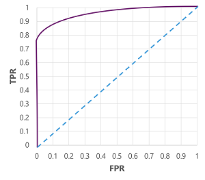
• The ROC curve for a perfect model would go up to TPR axis on the left and then across the FPR axis at the top.
• The available plot area for the curve is 1 X 1.
• Therefore, the area under this perfect curve will be 1.
• This means that the model is correct 100% of the time.
• In contrast the dotted line represents the results that would be achieved by randomly guessing a binary label; producing an area under the curve of 0.5.
• In other words, you could reasonably expect to guess correctly 50% of the time.
• In our case of diabetes model, the curve above is produced, and the Area Under the Curve metric is 0.875.
• Since the AUC is higher than 0.5, we can conclude that the model performs better at predicting whether or not a patient has diabetes than randomly guessing.

Multiclass Classification

• Multiclass classification is used to predict to which of the multiple possible classes an observation belongs.
• Since it is also a supervised ML technique, it follows the same iterative train, validate and evaluate process.

Sample Data

• Multiclass classification algorithms are used to calculate probability values for multiple class labels, enabling a model to predict the most probable class for a given observation.
• Following are some sample data for penguins.
• The data includes flipper length (Features, $\mathcal{X}$) of each penguin along with the penguin following species (Label, $\mathcal{Y}$).
  • 0: Adelie
  • 1: Gentoo
  • 2: Chinstrap

Flipper length (x)	Species (y)
167	0
172	0
225	2
197	1
189	1
232	2
158	0

Training a multiclass classification model

• To train a multiclass classification model, we need to use an algorithm to fit the training data to a function that calculates a probability value for each possible class.
• Following are the algorithms you can use to do this:
  • One-vs-Rest (OvR) algorithms
  • Multinomial algorithms.

One-vs-Rest (OvR) algorithms

• One-vs-Rest algorithms train a binary classification function for each class, each calculating the probability that the observation is an example of the target class.
• Each function calculates the probability of the observation being a specific class compared to any other class.
• In our case, the algorithm would create the following binary classification functions:
  • $f^0(\mathcal{X}) = P(\mathcal{Y}=0 | \mathcal{X})$
  • $f^1(\mathcal{X}) = P(\mathcal{Y}=1 | \mathcal{X})$
  • $f^2(\mathcal{X}) = P(\mathcal{Y}=2 | \mathcal{X})$ The probability that the outcome y equals k, given the input x.
• Each algorithm produces a sigmoid function that calculates a probability value between 0.0 and 1.0.
• A model trained using this kind of algorithm predicts the class for the function that produces the highest probability output.

Multinomial Algorithms

• The alternative approach is to use Multinomial Algorithms that create a single function that returns a multi-valued output.
• The output is a vector (an array of values) that contains the probability for all possible classes, with a probability score for each class which when totaled add up to 1. $f(\mathcal{X}) = [P(\mathcal{Y}=0|\mathcal{X}),P(\mathcal{Y}=1|\mathcal{X}),P(\mathcal{Y}=2|\mathcal{X})]$
• Regardless of which type of algorithm is used, the model uses the resulting function to determine the most probable class for a given set of featues ($\mathcal{X}$) and predicts the corresponding class label ($\mathcal{Y}$).

Evaluating a multiclass classification model

• Following is the sample data observed for a validated multiclass classifier.

Flipper length (x)	Actual species (y)	Predicted species (ŷ)
165	0	0
171	0	0
205	2	1
195	1	1
183	1	1
221	2	2
214	2	2

• The confusion matrix for a multclass classifier is similar to that of a binary classifier, except that it shows the number of predictions for each combination of predicted ($\hat{\mathcal{Y}}$) and the actual class labels ($\mathcal{Y}$).

From this confusion matrix we can determine the metrics for each individual class as follows:

Class	TP	TN	FP	FN	Accuracy	Recall	Precision	F1-Score
0	2	5	0	0	1.0	1.0	1.0	1.0
1	2	4	1	0	0.86	1.0	0.67	0.8
2	2	4	0	1	0.86	0.67	1.0	0.8

• To calculate the overall accuracy, recall, and precision metrics, you use the total of the TP, TN, FP, and FN metrics:
  • Overall accuracy = (13+6)÷(13+6+1+1) = 0.90
  • Overall recall = 6÷(6+1) = 0.86
  • Overall precision = 6÷(6+1) = 0.86
• The overall F1-score is calculated using the overall recall and precision metrics:
  • Overall F1-score = (2x0.86x0.86)÷(0.86+0.86) = 0.86

Clustering

• Clustering is a form of unsupervised ML in which observations as grouped into clusters based on similarities in data values or features.
• This kind of ML is called unsupervised because it does not make user of previously known label values to train a model.
• In clustering model, the label is the cluster to which the observation is assigned, based only on its features.

Sample Data

• Following is the sample data of flowers that records the number of leaves and petals on each flower.

• There are no known labels in the dataset.
• The goal is not to identify the species of each flower; but to group similar flowers together based on the number of leaves and petals.

Leaves ($\mathcal{X}_1$)	Petals ($\mathcal{X}_2$)
0	5
0	6
1	3
1	3
1	6
1	8
2	3
2	7
2	8

Training a clustering model

• There are multiple algorithms you can use for clustering.
• One of the most commonly used algorithms is K-Means clustering.
• It consists of the following steps:

Step 1:

1. The feature ($\mathcal{X}$) values are vectorized to define n-dimensional coordinates; where n is the number of features.
2. In the flower example, we have two features: Number of leaves ($\mathcal{X_1}$) and number of petals ($\mathcal{X_2}$).
3. Hence, the feature vector has 2 coordinates that we can use to conceptually plot the data points in two-dimensional space ($[\mathcal{X}_1,\mathcal{X}_2]$).

Step 2:

1. Now, you need to decide the number of clusters required.
2. This value is K.
3. Then K points are plotted at random coordinates.
4. These points become the center points for each cluster, so they are called centroids.

Step 3:

1. Each data point (in this case, flower) is assigned to its nearest centroid.

Step 4:

1. Each centroid is moved to the center of the data points assigned to it based on the mean distance between the points.

Step 5:

1. After the centroid is moved, the data points may now be closer to a different centroid.
2. Hence, the data points are reassigned to clusters based on the new closest centroid.

Step 6:

1. The centroid movement and the cluster reallocation steps are repeated until the clusters become stable or a predetermined maximum number of iterations is reached.

Evaluating a clustering model

• Since there is no known label with which to compare the predicted cluster assignment, evaluation of a clustering model is based on my well the resulting clusters are separated from one another.
• Following metrics can be used to evaluate this separation.
  • Average distance to cluster center: How close, on average, each point in the cluster is to the centroid of the cluster.
  • Average distance to other center: How close, on average, each point in the cluster is to the centroid of all other clusters.
  • Maximum distance to cluster center: The furthest distance between a point in the cluster and its centroid.
  • Silhouette: A value between -1 and 1 that summarizes the ratio of distance between points in the same cluster and points in different clusters (The closer to 1, the better the cluster separation).

Deep Learning

• Deep Learning is an advanced form of ML that tries to emulate the way human brain learns.
• The key to deep learning is the creation of artificial neural network that simulates electrochemical activity in biological neurons by using mathematical functions as should here.

Biological neural network	Artificial neural network
Neurons fire in response to electrochemical stimuli. When fired, the signal is passed to connected neurons.	Each neuron is a function that operates on an input value (x) and a weight (w). The function is wrapped in an activation function that determines whether to pass the output on.

• Artificial Neural Networks are made up of multiple layers of neurons

• It is like a deeply nested function.

• Due to such an architecture, this technique is referred to as deep learning and the models produced by it are often referred to as deep neural networks (DNNs).

• DNNs cal be used or many kinds of ML problems including regression and classification.

• More specialized DNNs can also be used for Natural Language Processing and Computer Vision.

• Just like other ML techniques discussed in this module, deep learning involves fitting some training data to a function that can predict the label ($\mathcal{Y}$) based on the value of one or more features ($\mathcal{X}$).

• The function ($f(\mathcal{X})$) is the outer layer of the nested function in which each layer of the neural network encapsulates functions that operate on $\mathcal{X}$ and the weight $\mathcal{w}$ values associated with them.

• Lets visualize this iterative function, $f(\mathcal{X}) = f3(f2(f1(\mathcal{X})))$

• Each $fi()$ is a layer in the network.

• Considering a concrete example,

  • Input feature x = temperature
  • Output label y = 1 means "Turn on Cooler", y = 0 means "Open Window"

• Lets simulate a neural network with 3 layers, and each layer is a function.

def f1(x):  # Layer 1: Multiply input by weight and add bias
    w1 = 0.4
    b1 = 1.0
    return x * w1 + b1

def f2(x):  # Layer 2: Apply activation (ReLU)
    return max(0, x)

def f3(x):  # Layer 3: Final output using sigmoid
    import math
    return 1 / (1 + math.exp(-x))  # Sigmoid to get probability

• Now we define final nested function,

def f(x):
    return f3(f2(f1(x)))  # Apply layer 1, then 2, then 3

• Try with x = 30 temperature,

print(f(30))  # Should give a value between 0 and 1

• Here is a walk through of it.

x = 30
f1(30) = 30 * 0.4 + 1.0 = 13
f2(13) = max(0, 13) = 13  (ReLU passes it through)
f3(13) = 1 / (1 + e^-13) ≈ 0.999998  => Very likely to turn on the cooler

Sample Data

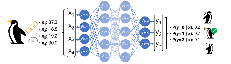
• Following is the example in which a neural network is used to define a classification model for penguin species.

• The feature data (x) consists of some measurements of a penguin. Specifically, the measurements are:

  • The length of the penguin's bill.
  • The depth of the penguin's bill.
  • The length of the penguin's flippers.
  • The penguin's weight.

• In this case, x is a vector of four values, or mathematically, $\mathcal{X}=[\mathcal{X}1,\mathcal{X}2,\mathcal{X}3,\mathcal{X}4]$.

• The label we are trying to predict (y) is the species of the penguin, and that there are three possible species it could be:

  • Adelie
  • Gentoo
  • Chinstrap

• This is an example of a classification problem, in which the ML model must predict the most probable class, to which an observation belongs.

• A classification model accomplishes this by predicting a label that consist of the probability for each class.

• In other words, y is a vector of three probability values; one for each possible classes: $[P(\mathcal{y}=0|\mathcal{x}), P(\mathcal{y}=1|\mathcal{x}), P(\mathcal{y}=2|\mathcal{x})]$

• The process of inferencing a predicted penguin class using this network is:

Step 1

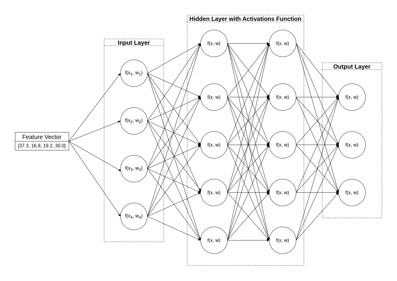
1. The feature vector for a penguin observation is fed into the input layer of the neural network.
2. This input layer consists of a neuron for each $\mathcal{X}$ value.
3. In this example, the following $\mathcal{X}$ vector is used as the input: [ 37.3, 16.8, 19.2, 30.0 ]

Step 2

1. Each functions on the first layer of neurons calculate a weighted sum by combining the $\mathcal{X}$ value and w weight.
2. This value is then passed to the activation function which further determines if the value meets the threshold to be passed to the next layer.

Step 3

1. Each neuron in the layer is connected to all the neurons in the next layer.
2. This architecture is sometimes called a fully connected network.
3. Therefore, the results of each layer are fed forward through the network until they reach the output layer.

Step 4

1. The output layer produces a vector of values.
2. In this case, it uses softmax or similar function to calculate the probability distribution for the three possible classes of penguin.
3. In this example the output vector is [0.2, 0.7, 0.1].

Step 5:

1. The elements of the vector produced by the output layer represent the probabilities for classes 0, 1 and 2.
2. Since the second value is the highest, so the model predicts that the species of the penguin is 1.

How does a Neural Network Learn?

• The weights in the neural network are central to how it calculates the predicted value for labels.
• During the training process, the model learn the weights that will result in the most accurate predictions.

Step 1:

1. The training and validation datasets are defined and the training features are fed into the input layer.

Step 2:

1. The neurons in each layer of the network apply their weights which are initially assigned randomly.
2. Further, the neurons feed the data through the network.

Step 3:

1. The output layer produces a vector containing the calculated values for $\hat{\mathcal{Y}}$.
2. For example, an output for a penguin class prediction might be [0.3, 0.1, 0.6].

Step 4:

1. A loss function is used to compare the predicted $\hat{\mathcal{Y}}$ values to known $\mathcal{Y}$ values and aggregate the difference which is known as loss.
2. For example, for the output in previous step, if we already know that the class is 2, then the $\mathcal{Y}$ should be [0.0, 0.0, 1.0].
3. Therefore, the absolute different between known class and predicted class is [0.3, 0.1, 0.4].
4. In reality the loss function calculates the aggregate variance for multiple cases and summarizes it as a single loss value. - The most common loss function to use, in this case is Categorical Cross-Entropy Loss. - The formula for this function is, $Loss = - \sum_{i=1}^{c}\mathcal{Y}_i . log(\hat{\mathcal{Y}_i})$ - Lets understand this formula. - First important thing that we need is to know how much is the different between the predicted class probability has actual class. - This difference is called Loss. - If the difference is 0, there is no loss and its perfect. If the difference is 0.2, the loss is small. If the difference is 0.6, the loss is medium and if the difference is 1, the loss is big. - Now to understand the loss, we need a formula that gives low values when the prediction is close to the true answer; whereas gives high value when the prediction is far off. - log is something that can help with this requirement because when the value is 1, its log value is 0, and as the value decreases to 0, its log value becomes increasingly negative. - This means that as the predicted value gets further from the true value, the log value increases exponentially, making the loss grow larger, which is exactly what we want when a prediction is farther from the true label. - Since the log values becomes negative, we have a negative sign in the formula to compensate. - Further, we multiply the log value of the predicted class probability so that we can eliminate all the other class probability since their actual value will be 0. - This is how, this loss formula helps us evaluate the networks.

Step 5:

1. Since the entire network is essentially one large nested function, differential calculus can be used to evaluate how the loss can be changed with respect to the change in weights $\frac{dL}{dw}$, resulting in optimizing the function.
2. The specific optimization technique can vary, but usually involves a gradient descent approach in which each weight is increased or decrease to minimize the loss.

Step 6:

1. The changes to the weights are backpropagated to the layers in the network, replacing the previously used values.

Step 7:

1. This process is repeated over multiple iterations, known as epochs, until the loss is minimized and the model predicts acceptably accurately.

note

While it's easier to think of each case in the training data being passed through the network one at a time, in reality, the data is batched into matrices and processed using linear algebraic calculations. For this reason, neural network training is best performed on computers with graphical processing units (GPUs) that are optimized for vector and matrix manipulation.

Transformers

• Today's generative AI applications are powered by language models, which are specialized type of ML model that you can use to perform NLP tasks, including
  • Determining sentiment or otherwise classifying natural language text.
  • Summarizing text.
  • Comparing multiple text sources for semantic similarity.
  • Generating new natural language.
• While the mathematical principles behind these language models can be complex, as basic understanding of the architecture used to implement them can help you gain a conceptual understanding of how they work.

Transformer Models

• Today's cutting edge LLMs are based on the transformer architecture.
• The transformer architecture is based on earlier successful models for understanding and working with words in NLP.
• It takes those ideas and improves them, especially to do language generation more effectively.
• Transformer models are trained with large volumes of text, enabling them to represent the semantic relationships between words, and use those relationships to determine probable sequences of text that make sense.
• Transformer models with a large enough vocabulary are capable of generating language responses that are tough to distinguish from human responses.
• Transformer model architecture consists of two components or blocks:
  • An encoder block that creates semantic relationships of the training vocabulary.
  • A decoder block that generates new language sequences.

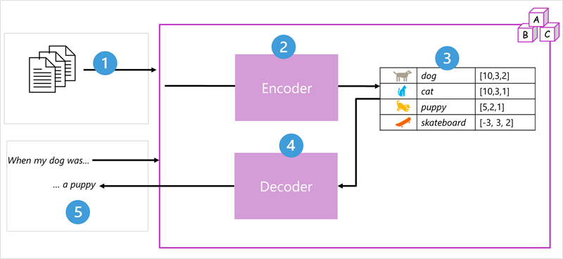
Step 1:

1. The model is trained with large volume of natural language text, often sourced from the internet or other public sources of text.

Step 2:

1. The sequences of text are broken down into tokens, for example, individual words.
2. The encoder block processes these token sequences using a technique called attention to determine relationships between tokens, for example, which tokens influence the presence of other tokens in a sequence, different tokens that are commonly used in the same context, and so on.

Step 3:

1. The output from the encoder is the collection of vectors.
2. The vectors are multi-valued numeric arrays in which each elements represents a semantic attribute of the tokens.
3. These vectors are referred to as embeddings.
4. To understand embeddings much better, I would recommend you to watch the following video by codebasics.

Step 4:

1. The decoder block works on a new sequence of text tokens and uses the embeddings generated by the encoder to generate an appropriate natural language output.

Step 5:

1. For example, given an input sequence like "When my dog was", the model can use the attention technique to analyze the input tokens and the semantic attributes encoded in the embeddings to predict an appropriate completion of the sentence, such as "a puppy".

• In practice, the specific implementations of the architecture vary.
• For example, the Bidirectional Encoder Representations from Transformers (BERT) model developed by Google to support their search engine uses only the encoder block, while the Generative Pretrained Transformer (GPT) model developed by OpenAI uses only the decoder block.

Tokenization

• The first step in training a transformer is the decompose the training text into tokens.
• In other words, identify the unique value for each text.
• For simplicity, consider each word in the training text as token.
• In reality, tokens can be generated for partial words or combination of words and punctuation.
• For example, consider the following text.
• "I heard a dog bark loudly at a cat."
• To tokenize the text, you can identify each discrete word and assign token IDs to them.

- I (1)
- heard (2)
- a (3)
- dog (4)
- bark (5)
- loudly (6)
- at (7)
- ("a" is already tokenized as 3)
- cat (8)

• The sentence can now be represented with tokens: { 1 2 3 4 5 6 7 3 8 }.
• Similarly, the sentence "I heard a cat" could be represented as { 1 2 3 8 }.
• As you continue to train the model, each new token in the training text is added to the vocabulary with appropriate token IDs.

- meow (9)
- skateboard (10)
- and so on...

• With a sufficient large set of training text, a vocabulary of many thousands of tokens could be compiled.

Embeddings

• While it may be convenient to represent tokens as simple IDs, essentially creating an index for all the words in the vocabulary, they dont tell us anything about the meaning of the words, or the relationship between them.

• To create vocabulary that encapsulates semantic relationship between the tokens, we define contextual vectors, known as embeddings, for them.

• Vectors are multi-valued numeric representations of information, for example, [10, 3, 1].

• In this representation, each numeric element represents a particular attribute of the information.

• If you watched the above linked video by codebasics, you will be able to understand what embeddings are.

• The specific categories for the element of the vectors, in a language model, are determined during training, based on how commonly words are used together or in similar contexts.

• Vectors represent lines in multidimensional space, describing direction and distance along multiple axes.

• Essentially think of the elements in an embedding vector as representing steps, along a path, in multidimensional space.

• For example, a vector with three elements represents a path in 3-dimensional space.

• The three values in this vector indicates the unit traveled forward/backward, left/right and up/down.

• Overall, the vector describes the direction and distance of the path from origin to end.

• Each element in the embeddings, represents some semantic attribute of the token.

• Therefore, semantically similar tokens results in vectors that have a similar orientation or in other words, they point in the same direction.

• A technique called "cosine similarity" is used to determine if two vectors have similar directions, regardless of distance.

• Now to understand what did we choose cosine similarity for determine, we need to understand some geometry.

• Basically, embeddings of each token, can be plotted into the graph with one line, since all the values in the embeddings basically are the values of each axes.

• Consider an example for the embeddings of following 2 words.

  • Love: [1, 5]
  • Like: [4, 4]

• Since there are only 2 values in the embeddings, we can plot it into a 2 dimentional graph as below.

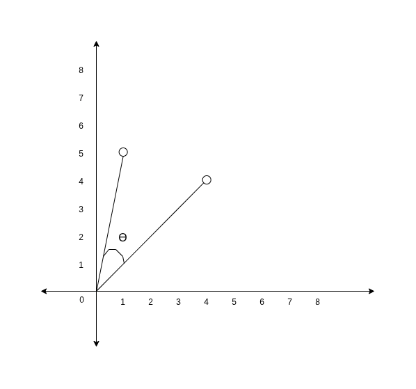
• Hence, essentially we converted embeddings of each token into lines.
• Now, consider the angle between these 2 lines is $\theta$.
• If we calculate the value of $cos(\theta)$, we get a value between -1 to 1.
• When you calculate $cos$ value of an angle between two lines, it essentially indicates, how closely, the two lines are aligned.
• If the angle between two lines is 0, that means the lines are one on the top of other, both the lines can be said to perfectly aligning.
• Hence the value of $cos(0)$ would be 1.
• If there is an angle of $90^o$, the value of $cos(90)$ would be 0, and for the angle of $180^o$, the value would be -1.
• Therefore calculating the cosine similarity between two embeddings helps us understand how close two tokens related to each other.
• Now, one issue in finding cosine similarity is that we first need to know the angle between the lines formed by the embeddings.
• While it might be possible if the embeddings have 2 to 3 values since we can plot 2 dimensional or 3 dimensional graph easily.
• For a multidimensional graph, we better look for a multiple that can help us calculate the cosine value of two lines formed by two embeddings.
• In euclidean space, the dot product of two non-zero vectors A and B is defined as: $$\vec{A}\cdot\vec{B} = \lvert\lvert\vec{A}\rvert\rvert\cdot\lvert\lvert\vec{B}\rvert\rvert\cdot\cos(\theta)$$
• Where,
  • $\vec{A}\cdot\vec{B}$ is the dot product of vectors A and B.
  • $\lvert\lvert\vec{A}\rvert\rvert$ and $\lvert\lvert\vec{B}\rvert\rvert$ are the magnitudes of vectors A and B.
  • $\theta$ is the angle between vectors A and B.
• This formula arises from the geometric definition of the dot product, relating it to the angle between the two vectors.
• Therefore, $$\cos(\theta) = \frac{\vec{A}\cdot\vec{B}}{\lvert\lvert\vec{A}\rvert\rvert\cdot\lvert\lvert\vec{B}\rvert\rvert}$$
• Simplifying it, $$\cos(\theta) = \frac{\sum^n_{i=1}A_iB_i}{\sqrt{\sum_{i=0}^nA_i^2\sum_{i=0}^nB_i^2}}$$
• As indicated earlier, the more the value of cosine similarity is near to 1, the more two vectors are similar and vise versa.

note

The previous example shows a simple example model in which each embedding has only two dimensions. Real language models have many more dimensions.

• There are multiple ways you can calculate appropriate embeddings for a given set of tokens, including language modeling algorithms like Word2Vec or the encoder block in a transformer model.

Attention

• The encoder and decoder block in a transformer model includes multiple layers that from the neural network for the model.

• We dont need to go into the details of all these layers, but its useful to consider one of the types of layers that is used in both blocks: attention layers.

• Attention is a technique used to examine a sequence of text tokens and try to quantify the strength of the relationships between them.

• In particular, self-attention involves considering how other tokens around one particular token influence that token's meaning.

• In an encoder block, each token is carefully examined in context, and an appropriate encoding is determined for its vector embedding.

• The vector values are based on the relationship between the token and other tokens with which it frequently appears.

• This contextualized approach means that the same word might have multiple embeddings depending on the context in which its used.

• For example, "The bark of a tree" means something different to "I heard a dog bark".

• To understand contextual embeddings much better, I would recommend you to watch the following video by codebasics. You may skip the tutorial if you want to.

• In a decoder block, attention layers are used to predict the next token in a sequence.

• For each token generated, the model has an attention layer that takes into account the sequence of tokens up to that point.

• The models considers which of the tokens are most influential when considering what the next token should be.

• For example, given the sequence "I heard a dog", the attention layer might assign a greated weight to the tokens "heard" and "dog" when considering the next work in the sequence.

• Remember the attention layer is working with numeric representations of the tokens, not the actual text.

• In a decoder, the process starts with a sequence of token embeddings representing the text to be completed.

• The first thing that happens if that another positional encoding layer adds a value to each embedding to indicate its position in the sequence, as follows:

- [**1**,5,6,2]  (I)
- [**2**,9,3,1]  (heard)
- [**3**,1,1,2]  (a)
- [**4**,10,3,2] (dog)

• During training, the goal is to predict the vector for the final token in the sequence based on the preceding tokens.

• When we are predicting the next token, since not all the previous words are that important, the attention layer assigns a numeric weight to each token in the sequence so far.

• It uses that value to perform a calculation on the weighted vectors that produces an attention score that can be used to calculate a possible vector for the next token.

• In practice, a technique called multi-head attention uses different elements of the embeddings to calculate multiple attention scores.

• A neural network is then used to evaluate all possible tokens to determine the most probable token with which to continue the sequence.

• The process continues iteratively for each token in the sequence, with the output sequence so far being used regressively as the input for the next iteration – essentially building the output one token at a time.

• The following animation shows a simplified representation of how this works – in reality, the calculations performed by the attention layer are more complex; but the principles can be simplified as shown:

Step 1

1. A sequence of token embeddings is fed into the attention layer.
2. Each token is represented as a vector of numeric values.

Step 2

1. The goal in a decoder is to predict the next token in the sequence.
2. This token will also be a vector that aligns to an embedding in the model’s vocabulary.

Step 3

1. The attention layer evaluates the sequence so far and assigns weights to each token to represent their relative influence on the next token.

Step 4

1. The weights can be used to compute a new vector for the next token with an attention score.
2. Multi-head attention uses different elements in the embeddings to calculate multiple alternative tokens.

Step 5

1. A fully connected neural network uses the scores in the calculated vectors to predict the most probable token from the entire vocabulary.

Step 6

1. The predicted output is appended to the sequence so far, which is used as the input for the next iteration.

• During training, the actual sequence of tokens is known.

• We just mask the ones that come later in the sequence than the token position currently being considered.

• Same as other neural network, the predicted value for the token vector is compared to the actual value of the next vector in the sequence and the loss is calculated.

• The weights are then incrementally adjusted to reduce the loss and improve the model.

• When used for inferencing (predicting a new sequence of tokens), the trained attention layer applies weights that predict the most probable token in the model’s vocabulary that is semantically aligned to the sequence so far.

• What all of this means, is that a transformer model such as GPT-4 (the model behind ChatGPT and Bing) is designed to take in a text input (called a prompt) and generate a syntactically correct output (called a completion).

• In effect, the "magic" of the model is that it has the ability to string a coherent sentence together.

• This ability doesn't imply any "knowledge" or "intelligence" on the part of the model; just a large vocabulary and the ability to generate meaningful sequences of words.

• What makes an LLM like GPT-4 so powerful however, is the sheer volume of data with which it has been trained (public and licensed data from the Internet) and the complexity of the network.

• This enables the model to generate completions that are based on the relationships between words in the vocabulary on which the model was trained; often generating output that is indistinguishable from a human response to the same prompt.

Automated Machine Learning in Azure Machine Learning

• Complete the lab to explore the automated machine learning capability in Azure Machine Learning Studio and use it to train and evaluate a machine learning model.